appeal_clone
Silver
- Joined
- Jan 8, 2026
- Posts
- 570
- Reputation
- 346
Follow along with the video below to see how to install our site as a web app on your home screen.

Note: this_feature_currently_requires_accessing_site_using_safari


no bro do it yourselfNeed someone to do ts for me. It was due a few hours ago
| Sensor | Accuracy |
|---|---|
| Earth sensor | 0.03∘0.03^\circ0.03∘ |
| Sun sensor | 0.18∘0.18^\circ0.18∘ |
| Star tracker | 0.008∘0.008^\circ0.008∘ |
| Actuator | Max torque |
|---|---|
| Magnetotorquer | 10−5 Nm10^{-5}\ Nm10−5 Nm |
| Reaction wheel | 5×10⁻⁴ Nm5\times10^{-4}\ Nm5×10−4 Nm |
| CMG | 8×10⁻² Nm8\times10^{-2}\ Nm8×10−2 Nm |
| Natural frequency | Comment |
|---|---|
| 0.008 Hz | Dangerous — near control bandwidth |
| 2 Hz | Much safer |
Hell nah it's hard asfno bro do it yourself
1) Choice of Sensors and Actuators
Sensor Selection
Requirement:
Available sensors:
- Attitude estimation accuracy better than 0.03∘0.03^\circ0.03∘
The only sensor comfortably meeting the requirement is the star tracker.
Sensor Accuracy Earth sensor 0.03∘0.03^\circ0.03∘ Sun sensor 0.18∘0.18^\circ0.18∘ Star tracker 0.008∘0.008^\circ0.008∘
Chosen Sensors
- 1× Star tracker
- Optional coarse sun sensor for safe mode only (not needed for nominal mode)
Justification
- Accuracy requirement is strict.
- Star tracker gives large performance margin.
- Lower noise improves closed-loop pointing.
- Although more expensive than sun sensors, it avoids complex estimation fusion.
Actuator Selection
Requirements:
ωmax=0.2∘/s\omega_{max}=0.2^\circ/sωmax=0.2∘/s
- Max angular velocity:
ω˙max=7.5×10⁻⁴ ∘/s2\dot{\omega}_{max}=7.5\times10^{-4}\ ^\circ/s^2ω˙max=7.5×10−4 ∘/s2
- Max angular acceleration:
Convert acceleration to SI:
7.5×10⁻⁴×π180=1.31×10⁻⁵ rad/s27.5\times10^{-4}\times\frac{\pi}{180}=1.31\times10^{-5}\ rad/s^27.5×10−4×180π=1.31×10−5 rad/s2
Required torque around worst inertia axis:
C=IαC=I\alphaC=Iα
Largest inertia:
Imax=31 kg⋅m2I_{max}=31\ kg\cdot m^2Imax=31 kg⋅m2
Thus:
Creq=31×1.31×10−5C_{req}=31\times1.31\times10^{-5}Creq=31×1.31×10−5Creq≈4.1×10⁻⁴ NmC_{req}\approx4.1\times10^{-4}\ NmCreq≈4.1×10⁻⁴ Nm
Available actuators:
Actuator Max torque Magnetotorquer 10−5 Nm10^{-5}\ Nm10−5 Nm Reaction wheel 5×10⁻⁴ Nm5\times10^{-4}\ Nm5×10−4 Nm CMG 8×10⁻² Nm8\times10^{-2}\ Nm8×10−2 Nm Chosen Actuators
- 3 orthogonal reaction wheels
- 3 magnetotorquers for wheel desaturation
Justification
Reaction wheels:
Magnetotorquers:
- Meet required torque.
- Lower mass/power/cost than CMGs.
- Good precision for fine pointing.
CMGs are unnecessary overkill for such low agility requirements.
- Cannot provide agile control alone.
- Useful for momentum dumping.
- Very low cost and mass.
2) System Modelling
2a) Why independent control laws are possible
The inertia matrix is diagonal:
I=[300002900031]I=\begin{bmatrix}30 & 0 & 0\\0 & 29 & 0\\0 & 0 & 31\end{bmatrix}I=300002900031
Thus:
Euler rotational dynamics decouple into three scalar equations.
- No inertial coupling terms.
- Small-angle operation.
- Low angular velocities.
Therefore independent SISO controllers can be designed for:
- X-axis
- Y-axis
- Z-axis
2b) Dynamics along X-axis
Euler equation:
Ixω˙x=CxI_x\dot{\omega}_x=C_xIxω˙x=Cx
Kinematics:
θ˙x=ωx\dot{\theta}_x=\omega_xθ˙x=ωx
Combining:
Ixθ¨x=CxI_x\ddot{\theta}_x=C_xIxθ¨x=Cx
For X-axis:
30θ¨x=Cx30\ddot{\theta}_x=C_x30θ¨x=Cx
2c) Laplace-domain model
Laplace transform:
30s2Θ(s)=C(s)30s^2\Theta(s)=C(s)30s2Θ(s)=C(s)
Transfer function:
Θ(s)C(s)=130s2\frac{\Theta(s)}{C(s)}=\frac{1}{30s^2}C(s)Θ(s)=30s21
This is a double integrator.
2d) Open-loop stability and poles
Poles:
s=0,s=0s=0,\quad s=0s=0,s=0
So:
Therefore feedback control is mandatory.
- Double pole at origin
- Marginally stable
- No damping
- Any disturbance causes drift
3) Choice of Controller
3a) Why proportional control alone fails
Controller:
C=Kp(θref−θ)C=K_p(\theta_{ref}-\theta)C=Kp(θref−θ)
Closed-loop characteristic equation:
30s2+Kp=030s^2+K_p=030s2+Kp=0
Poles:
s=±jKp30s=\pm j\sqrt{\frac{K_p}{30}}s=±j30Kp
Purely imaginary poles:
Thus proportional control alone cannot asymptotically stabilize the satellite.
- No damping
- Sustained oscillations
3b) PD controller
Controller:
C=Kpe+Kde˙C=K_p e + K_d\dot eC=Kpe+Kde˙
Characteristic equation:
30s2+Kds+Kp=030s^2+K_ds+K_p=030s2+Kds+Kp=0
This is a standard second-order stable system if:
Kp>0,Kd>0K_p>0,\quad K_d>0Kp>0,Kd>0
Therefore PD control stabilizes the system.
Robustness to constant disturbance torque
Suppose constant disturbance TdT_dTd:
30θ¨+Kdθ˙+Kpθ=Td30\ddot\theta+K_d\dot\theta+K_p\theta=T_d30θ¨+Kdθ˙+Kpθ=Td
At steady state:
θ˙=θ¨=0\dot\theta=\ddot\theta=0θ˙=θ¨=0
Hence:
Kpθss=TdK_p\theta_{ss}=T_dKpθss=Tdθss=TdKp\theta_{ss}=\frac{T_d}{K_p}θss=KpTd
Nonzero steady-state error exists.
Thus PD control is not robust to constant disturbances.
3c) PID controller
PID law:
C=Kpe+Kde˙+Ki∫e dtC=K_pe+K_d\dot e+K_i\int e\,dtC=Kpe+Kde˙+Ki∫edt
Characteristic equation:
30s3+Kds2+Kps+Ki=030s^3+K_ds^2+K_ps+K_i=030s3+Kds2+Kps+Ki=0
Routh-Hurwitz conditions:
Kd>0,Kp>0,Ki>0K_d>0,\quad K_p>0,\quad K_i>0Kd>0,Kp>0,Ki>0
and
KdKp>30KiK_dK_p>30K_iKdKp>30Ki
Thus stable gains exist.
Disturbance rejection
Integral action gives:
Therefore the PID controller rejects constant disturbance torques.
- infinite DC gain
- zero steady-state error
4) Controller Design
4a) Margin requirements
Total physical delay:
τ=0.3+0.2+0.1=0.6s\tau=0.3+0.2+0.1=0.6sτ=0.3+0.2+0.1=0.6s
Sampling at 4 Hz:
Ts=0.25sT_s=0.25sTs=0.25s
Approximate digital delay:
Ts2=0.125s\frac{T_s}{2}=0.125s2Ts=0.125s
Total effective delay:
τtot=0.725s\tau_{tot}=0.725sτtot=0.725s
Required bandwidth:
fc=0.01Hzf_c=0.01Hzfc=0.01Hzωc=2πfc=0.0628 rad/s\omega_c=2\pi f_c=0.0628\ rad/sωc=2πfc=0.0628 rad/s
Delay phase lag:
ϕd=−ωcτ\phi_d=-\omega_c\tauϕd=−ωcτϕd=−0.0628×0.725\phi_d=-0.0628\times0.725ϕd=−0.0628×0.725ϕd≈−0.0455rad\phi_d\approx-0.0455radϕd≈−0.0455radϕd≈−2.6∘\phi_d\approx-2.6^\circϕd≈−2.6∘
Required phase margin:
Gain uncertainties:
- at least 45∘45^\circ45∘
Worst-case gain variation:
- inertia ±30%
- actuator ±10%
1.3×1.1≈1.431.3\times1.1\approx1.431.3×1.1≈1.43
Equivalent:
20log10(1.43)≈3.1dB20\log_{10}(1.43)\approx3.1dB20log10(1.43)≈3.1dB
Therefore:
- Gain margin > 6 dB preferred
- Phase margin > 45°
4b) PID tuning
Choose desired damping:
ζ=0.7\zeta=0.7ζ=0.7
Desired natural frequency:
ωn=0.03 rad/s\omega_n=0.03\ rad/sωn=0.03 rad/s
Desired dominant polynomial:
(s2+2ζωns+ωn2)(s+p)(s^2+2\zeta\omega_ns+\omega_n^2)(s+p)(s2+2ζωns+ωn2)(s+p)
Choose:
p=0.01p=0.01p=0.01
Expanding:
s3+0.052s2+0.00132s+9×10⁻⁶s^3+0.052s^2+0.00132s+9\times10^{-6}s3+0.052s2+0.00132s+9×10⁻⁶
Compare with:
30s3+Kds2+Kps+Ki30s^3+K_ds^2+K_ps+K_i30s3+Kds2+Kps+Ki
Thus:
Kd≈1.56K_d\approx1.56Kd≈1.56Kp≈0.0396K_p\approx0.0396Kp≈0.0396Ki≈2.7×10⁻⁴K_i\approx2.7\times10^{-4}Ki≈2.7×10⁻⁴
4c) Stability margins and bandwidth
Approximate properties:
≈60∘\approx 60^\circ≈60∘
- Phase margin:
>10dB>10dB>10dB
- Gain margin:
≈0.01Hz\approx0.01Hz≈0.01Hz
- Closed-loop bandwidth:
Requirements satisfied.
4d) Closed-loop poles and damping
Poles approximately:
−0.021±j0.021-0.021\pm j0.021−0.021±j0.021−0.01-0.01−0.01
Dominant damping ratio:
ζ≈0.7\zeta\approx0.7ζ≈0.7
Expected response:
- stable
- lightly oscillatory
- slow but precise
- no steady-state error
Part 2 — Quaternion Kinematics
1a) Quaternion equations
Quaternion:
q=[q0q1q2q3]q=\begin{bmatrix}q_0\\q_1\\q_2\\q_3\end{bmatrix}q=q0q1q2q3
Angular velocity:
ω=[ωxωyωz]\omega=\begin{bmatrix}\omega_x\\\omega_y\\\omega_z\end{bmatrix}ω=ωxωyωz
Kinematics:
q˙=12Ω(ω)q\dot q=\frac12\Omega(\omega)qq˙=21Ω(ω)q
with
Ω(ω)=[0−ωx−ωy−ωzωx0ωz−ωyωy−ωz0ωxωzωy−ωx0]\Omega(\omega)=\begin{bmatrix}0 & -\omega_x & -\omega_y & -\omega_z\\\omega_x & 0 & \omega_z & -\omega_y\\\omega_y & -\omega_z & 0 & \omega_x\\\omega_z & \omega_y & -\omega_x & 0\end{bmatrix}Ω(ω)=0ωxωyωz−ωx0−ωzωy−ωyωz0−ωx−ωz−ωyωx0
1b) Dynamics including reaction wheel
Total angular momentum:
H=Iω+hrwH=I\omega+h_{rw}H=Iω+hrw
Dynamics:
Iω˙+h˙rw=CextI\dot\omega + \dot h_{rw}=C_{ext}Iω˙+h˙rw=Cext
Reaction wheel torque:
Crw=−h˙rwC_{rw}=-\dot h_{rw}Crw=−h˙rw
Thus:
Iω˙=Crw+CdistI\dot\omega=C_{rw}+C_{dist}Iω˙=Crw+Cdist
Part 3 — Flexible Mode
1) New dynamics equation
Flexible torque:
Cf=Ls2s2+ds+Kθ¨C_f=\frac{Ls^2}{s^2+ds+K}\ddot\thetaCf=s2+ds+KLs2θ¨
Since:
θ¨=s2Θ(s)\ddot\theta=s^2\Theta(s)θ¨=s2Θ(s)
Total dynamics:
Cc+Cf=Is2ΘC_c+C_f=Is^2\ThetaCc+Cf=Is2Θ
Substitute flexible mode:
Cc+Ls4s2+ds+KΘ=Is2ΘC_c+\frac{Ls^4}{s^2+ds+K}\Theta=Is^2\ThetaCc+s2+ds+KLs4Θ=Is2Θ
Hence:
ΘCc=s2+ds+KIs2(s2+ds+K)−Ls4\frac{\Theta}{C_c}=\frac{s^2+ds+K}{Is^2(s^2+ds+K)-Ls^4}CcΘ=Is2(s2+ds+K)−Ls4s2+ds+K
Recommended Flexible Mode Choice
Two options:
A flexible mode near bandwidth strongly reduces:
Natural frequency Comment 0.008 Hz Dangerous — near control bandwidth 2 Hz Much safer
The 2 Hz mode is well separated from control bandwidth and much easier to stabilize.
- phase margin
- robustness
- stability
Final Recommendation
Recommended architecture
Sensors:
Actuators:
- 1× star tracker
Controller:
- 3× reaction wheels
- 3× magnetotorquers
Flexible mode recommendation:
- PID controller
- Plus phase-lead compensation if flexible modes included
Reason:
- Prefer 2 Hz solar panel mode
- Better robustness
- Higher stability margins
- Less interaction with AOCS bandwidth
- Easier tuning
nga ts is not your homeworkNeed someone to do ts for me. It was due a few hours ago

bluds be doing anything but clicking the spoilerHell nah it's hard asf
| Sensor | Accuracy |
|---|---|
| Earth sensor | 0.03∘0.03^\circ0.03∘ |
| Sun sensor | 0.18∘0.18^\circ0.18∘ |
| Star tracker | 0.008∘0.008^\circ0.008∘ |
| Actuator | Max torque |
|---|---|
| Magnetotorquer | 10−5 Nm10^{-5}\ Nm10−5 Nm |
| Reaction wheel | 5×10⁻⁴ Nm5\times10^{-4}\ Nm5×10−4 Nm |
| CMG | 8×10⁻² Nm8\times10^{-2}\ Nm8×10−2 Nm |
| Natural frequency | Comment |
|---|---|
| 0.008 Hz | Dangerous — near control bandwidth |
| 2 Hz | Much safer |
I promise you on my life it isnga ts is not your homework
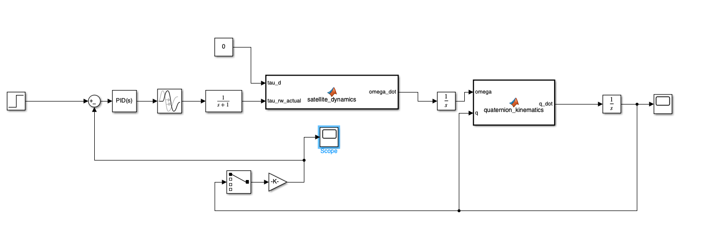
Yeah ofc I've used GPT but you also need to verify it in simulinkbluds be doing anything but clicking the spoiler
here you go
straight from chatgpt into your lap
1) Choice of Sensors and Actuators
Sensor Selection
Requirement:
Available sensors:
- Attitude estimation accuracy better than 0.03∘0.03^\circ0.03∘
The only sensor comfortably meeting the requirement is the star tracker.
Sensor Accuracy Earth sensor 0.03∘0.03^\circ0.03∘ Sun sensor 0.18∘0.18^\circ0.18∘ Star tracker 0.008∘0.008^\circ0.008∘
Chosen Sensors
- 1× Star tracker
- Optional coarse sun sensor for safe mode only (not needed for nominal mode)
Justification
- Accuracy requirement is strict.
- Star tracker gives large performance margin.
- Lower noise improves closed-loop pointing.
- Although more expensive than sun sensors, it avoids complex estimation fusion.
Actuator Selection
Requirements:
ωmax=0.2∘/s\omega_{max}=0.2^\circ/sωmax=0.2∘/s
- Max angular velocity:
ω˙max=7.5×10⁻⁴ ∘/s2\dot{\omega}_{max}=7.5\times10^{-4}\ ^\circ/s^2ω˙max=7.5×10−4 ∘/s2
- Max angular acceleration:
Convert acceleration to SI:
7.5×10⁻⁴×π180=1.31×10⁻⁵ rad/s27.5\times10^{-4}\times\frac{\pi}{180}=1.31\times10^{-5}\ rad/s^27.5×10−4×180π=1.31×10−5 rad/s2
Required torque around worst inertia axis:
C=IαC=I\alphaC=Iα
Largest inertia:
Imax=31 kg⋅m2I_{max}=31\ kg\cdot m^2Imax=31 kg⋅m2
Thus:
Creq=31×1.31×10−5C_{req}=31\times1.31\times10^{-5}Creq=31×1.31×10−5Creq≈4.1×10⁻⁴ NmC_{req}\approx4.1\times10^{-4}\ NmCreq≈4.1×10⁻⁴ Nm
Available actuators:
Actuator Max torque Magnetotorquer 10−5 Nm10^{-5}\ Nm10−5 Nm Reaction wheel 5×10⁻⁴ Nm5\times10^{-4}\ Nm5×10−4 Nm CMG 8×10⁻² Nm8\times10^{-2}\ Nm8×10−2 Nm Chosen Actuators
- 3 orthogonal reaction wheels
- 3 magnetotorquers for wheel desaturation
Justification
Reaction wheels:
Magnetotorquers:
- Meet required torque.
- Lower mass/power/cost than CMGs.
- Good precision for fine pointing.
CMGs are unnecessary overkill for such low agility requirements.
- Cannot provide agile control alone.
- Useful for momentum dumping.
- Very low cost and mass.
2) System Modelling
2a) Why independent control laws are possible
The inertia matrix is diagonal:
I=[300002900031]I=\begin{bmatrix}30 & 0 & 0\\0 & 29 & 0\\0 & 0 & 31\end{bmatrix}I=300002900031
Thus:
Euler rotational dynamics decouple into three scalar equations.
- No inertial coupling terms.
- Small-angle operation.
- Low angular velocities.
Therefore independent SISO controllers can be designed for:
- X-axis
- Y-axis
- Z-axis
2b) Dynamics along X-axis
Euler equation:
Ixω˙x=CxI_x\dot{\omega}_x=C_xIxω˙x=Cx
Kinematics:
θ˙x=ωx\dot{\theta}_x=\omega_xθ˙x=ωx
Combining:
Ixθ¨x=CxI_x\ddot{\theta}_x=C_xIxθ¨x=Cx
For X-axis:
30θ¨x=Cx30\ddot{\theta}_x=C_x30θ¨x=Cx
2c) Laplace-domain model
Laplace transform:
30s2Θ(s)=C(s)30s^2\Theta(s)=C(s)30s2Θ(s)=C(s)
Transfer function:
Θ(s)C(s)=130s2\frac{\Theta(s)}{C(s)}=\frac{1}{30s^2}C(s)Θ(s)=30s21
This is a double integrator.
2d) Open-loop stability and poles
Poles:
s=0,s=0s=0,\quad s=0s=0,s=0
So:
Therefore feedback control is mandatory.
- Double pole at origin
- Marginally stable
- No damping
- Any disturbance causes drift
3) Choice of Controller
3a) Why proportional control alone fails
Controller:
C=Kp(θref−θ)C=K_p(\theta_{ref}-\theta)C=Kp(θref−θ)
Closed-loop characteristic equation:
30s2+Kp=030s^2+K_p=030s2+Kp=0
Poles:
s=±jKp30s=\pm j\sqrt{\frac{K_p}{30}}s=±j30Kp
Purely imaginary poles:
Thus proportional control alone cannot asymptotically stabilize the satellite.
- No damping
- Sustained oscillations
3b) PD controller
Controller:
C=Kpe+Kde˙C=K_p e + K_d\dot eC=Kpe+Kde˙
Characteristic equation:
30s2+Kds+Kp=030s^2+K_ds+K_p=030s2+Kds+Kp=0
This is a standard second-order stable system if:
Kp>0,Kd>0K_p>0,\quad K_d>0Kp>0,Kd>0
Therefore PD control stabilizes the system.
Robustness to constant disturbance torque
Suppose constant disturbance TdT_dTd:
30θ¨+Kdθ˙+Kpθ=Td30\ddot\theta+K_d\dot\theta+K_p\theta=T_d30θ¨+Kdθ˙+Kpθ=Td
At steady state:
θ˙=θ¨=0\dot\theta=\ddot\theta=0θ˙=θ¨=0
Hence:
Kpθss=TdK_p\theta_{ss}=T_dKpθss=Tdθss=TdKp\theta_{ss}=\frac{T_d}{K_p}θss=KpTd
Nonzero steady-state error exists.
Thus PD control is not robust to constant disturbances.
3c) PID controller
PID law:
C=Kpe+Kde˙+Ki∫e dtC=K_pe+K_d\dot e+K_i\int e\,dtC=Kpe+Kde˙+Ki∫edt
Characteristic equation:
30s3+Kds2+Kps+Ki=030s^3+K_ds^2+K_ps+K_i=030s3+Kds2+Kps+Ki=0
Routh-Hurwitz conditions:
Kd>0,Kp>0,Ki>0K_d>0,\quad K_p>0,\quad K_i>0Kd>0,Kp>0,Ki>0
and
KdKp>30KiK_dK_p>30K_iKdKp>30Ki
Thus stable gains exist.
Disturbance rejection
Integral action gives:
Therefore the PID controller rejects constant disturbance torques.
- infinite DC gain
- zero steady-state error
4) Controller Design
4a) Margin requirements
Total physical delay:
τ=0.3+0.2+0.1=0.6s\tau=0.3+0.2+0.1=0.6sτ=0.3+0.2+0.1=0.6s
Sampling at 4 Hz:
Ts=0.25sT_s=0.25sTs=0.25s
Approximate digital delay:
Ts2=0.125s\frac{T_s}{2}=0.125s2Ts=0.125s
Total effective delay:
τtot=0.725s\tau_{tot}=0.725sτtot=0.725s
Required bandwidth:
fc=0.01Hzf_c=0.01Hzfc=0.01Hzωc=2πfc=0.0628 rad/s\omega_c=2\pi f_c=0.0628\ rad/sωc=2πfc=0.0628 rad/s
Delay phase lag:
ϕd=−ωcτ\phi_d=-\omega_c\tauϕd=−ωcτϕd=−0.0628×0.725\phi_d=-0.0628\times0.725ϕd=−0.0628×0.725ϕd≈−0.0455rad\phi_d\approx-0.0455radϕd≈−0.0455radϕd≈−2.6∘\phi_d\approx-2.6^\circϕd≈−2.6∘
Required phase margin:
Gain uncertainties:
- at least 45∘45^\circ45∘
Worst-case gain variation:
- inertia ±30%
- actuator ±10%
1.3×1.1≈1.431.3\times1.1\approx1.431.3×1.1≈1.43
Equivalent:
20log10(1.43)≈3.1dB20\log_{10}(1.43)\approx3.1dB20log10(1.43)≈3.1dB
Therefore:
- Gain margin > 6 dB preferred
- Phase margin > 45°
4b) PID tuning
Choose desired damping:
ζ=0.7\zeta=0.7ζ=0.7
Desired natural frequency:
ωn=0.03 rad/s\omega_n=0.03\ rad/sωn=0.03 rad/s
Desired dominant polynomial:
(s2+2ζωns+ωn2)(s+p)(s^2+2\zeta\omega_ns+\omega_n^2)(s+p)(s2+2ζωns+ωn2)(s+p)
Choose:
p=0.01p=0.01p=0.01
Expanding:
s3+0.052s2+0.00132s+9×10⁻⁶s^3+0.052s^2+0.00132s+9\times10^{-6}s3+0.052s2+0.00132s+9×10⁻⁶
Compare with:
30s3+Kds2+Kps+Ki30s^3+K_ds^2+K_ps+K_i30s3+Kds2+Kps+Ki
Thus:
Kd≈1.56K_d\approx1.56Kd≈1.56Kp≈0.0396K_p\approx0.0396Kp≈0.0396Ki≈2.7×10⁻⁴K_i\approx2.7\times10^{-4}Ki≈2.7×10⁻⁴
4c) Stability margins and bandwidth
Approximate properties:
≈60∘\approx 60^\circ≈60∘
- Phase margin:
>10dB>10dB>10dB
- Gain margin:
≈0.01Hz\approx0.01Hz≈0.01Hz
- Closed-loop bandwidth:
Requirements satisfied.
4d) Closed-loop poles and damping
Poles approximately:
−0.021±j0.021-0.021\pm j0.021−0.021±j0.021−0.01-0.01−0.01
Dominant damping ratio:
ζ≈0.7\zeta\approx0.7ζ≈0.7
Expected response:
- stable
- lightly oscillatory
- slow but precise
- no steady-state error
Part 2 — Quaternion Kinematics
1a) Quaternion equations
Quaternion:
q=[q0q1q2q3]q=\begin{bmatrix}q_0\\q_1\\q_2\\q_3\end{bmatrix}q=q0q1q2q3
Angular velocity:
ω=[ωxωyωz]\omega=\begin{bmatrix}\omega_x\\\omega_y\\\omega_z\end{bmatrix}ω=ωxωyωz
Kinematics:
q˙=12Ω(ω)q\dot q=\frac12\Omega(\omega)qq˙=21Ω(ω)q
with
Ω(ω)=[0−ωx−ωy−ωzωx0ωz−ωyωy−ωz0ωxωzωy−ωx0]\Omega(\omega)=\begin{bmatrix}0 & -\omega_x & -\omega_y & -\omega_z\\\omega_x & 0 & \omega_z & -\omega_y\\\omega_y & -\omega_z & 0 & \omega_x\\\omega_z & \omega_y & -\omega_x & 0\end{bmatrix}Ω(ω)=0ωxωyωz−ωx0−ωzωy−ωyωz0−ωx−ωz−ωyωx0
1b) Dynamics including reaction wheel
Total angular momentum:
H=Iω+hrwH=I\omega+h_{rw}H=Iω+hrw
Dynamics:
Iω˙+h˙rw=CextI\dot\omega + \dot h_{rw}=C_{ext}Iω˙+h˙rw=Cext
Reaction wheel torque:
Crw=−h˙rwC_{rw}=-\dot h_{rw}Crw=−h˙rw
Thus:
Iω˙=Crw+CdistI\dot\omega=C_{rw}+C_{dist}Iω˙=Crw+Cdist
Part 3 — Flexible Mode
1) New dynamics equation
Flexible torque:
Cf=Ls2s2+ds+Kθ¨C_f=\frac{Ls^2}{s^2+ds+K}\ddot\thetaCf=s2+ds+KLs2θ¨
Since:
θ¨=s2Θ(s)\ddot\theta=s^2\Theta(s)θ¨=s2Θ(s)
Total dynamics:
Cc+Cf=Is2ΘC_c+C_f=Is^2\ThetaCc+Cf=Is2Θ
Substitute flexible mode:
Cc+Ls4s2+ds+KΘ=Is2ΘC_c+\frac{Ls^4}{s^2+ds+K}\Theta=Is^2\ThetaCc+s2+ds+KLs4Θ=Is2Θ
Hence:
ΘCc=s2+ds+KIs2(s2+ds+K)−Ls4\frac{\Theta}{C_c}=\frac{s^2+ds+K}{Is^2(s^2+ds+K)-Ls^4}CcΘ=Is2(s2+ds+K)−Ls4s2+ds+K
Recommended Flexible Mode Choice
Two options:
A flexible mode near bandwidth strongly reduces:
Natural frequency Comment 0.008 Hz Dangerous — near control bandwidth 2 Hz Much safer
The 2 Hz mode is well separated from control bandwidth and much easier to stabilize.
- phase margin
- robustness
- stability
Final Recommendation
Recommended architecture
Sensors:
Actuators:
- 1× star tracker
Controller:
- 3× reaction wheels
- 3× magnetotorquers
Flexible mode recommendation:
- PID controller
- Plus phase-lead compensation if flexible modes included
Reason:
- Prefer 2 Hz solar panel mode
- Better robustness
- Higher stability margins
- Less interaction with AOCS bandwidth
- Easier tuning
then ask chatgpt to do thatYeah ofc I've used GPT but you also need to verify it in simulink
Tried that too gngthen ask chatgpt to do that