





Seth Walsh

Iconoclast
Contributor
- Joined
- Jan 12, 2020
- Posts
- 11,243
- Reputation
- 23,011
Multiplicative randomness continuously separates trajectories, and arithmetic averages increasingly become descriptions of the extreme right tail rather than descriptions of ordinary people.
In wealth dynamics, the mean becomes more and more prosperous while becoming less and less representative of almost anyone actually living inside the system.
This explains individual economic decay as ensemble statistics look "better".
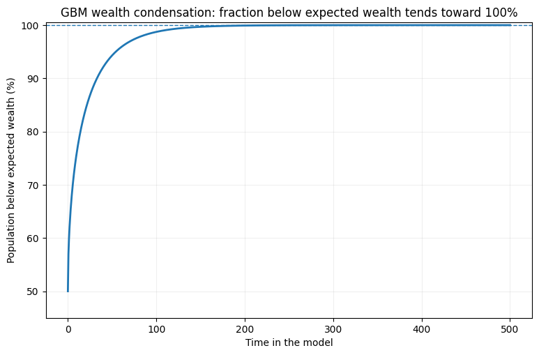
The first graph is the most important. At the beginning, about half the population is below the expected wealth level. As the multiplicative process runs, that proportion rises.
Why?
Because the distribution is not merely moving. It is stretching.
Imagine everyone begins here:
Time 0
●●●●●●●●●●●●●●●●●●●●
roughly equal
Then everyone receives independent percentage gains and losses.
After some time:
Later
●●●●●●●●●●●●●●● ●● ● ●
poor / ordinary rich very rich
Much later:
Much later
●●●●●●●●●●●●●●●●●●●●●●●●● ● ● ●
almost everyone extreme tail
The huge conceptual point is that wealth is multiplicative.
Suppose two people both get lucky.
One currently has €10.
One currently has €10 million.
A 20% positive shock gives the first person €2.
It gives the second person €2 million.
So once trajectories separate, subsequent percentage changes occur on radically different bases.
The distribution therefore keeps broadening.
And because wealth cannot symmetrically extend below zero in this simple model, the broadening becomes extraordinarily skewed in ordinary euro terms.
In log-wealth space, the distribution looks much more like a symmetric bell.
But when you transform back into actual wealth, the right-hand tail gets stretched enormously.
That is the central geometry:
LOG WEALTH
/\
/ \
/ \
_______/____________\_______
fairly symmetric
becomes something like:
ACTUAL WEALTH
███████████████████▇▆▅▄▃▂▂▁▁▁▁.........................tiny tail
but tail values are ENORMOUS
Most people occupy the dense mass on the left.
Very few people occupy the far-right tail.
But the far-right values become so enormous that they dominate the arithmetic average.
And that brings us to the third graphic.
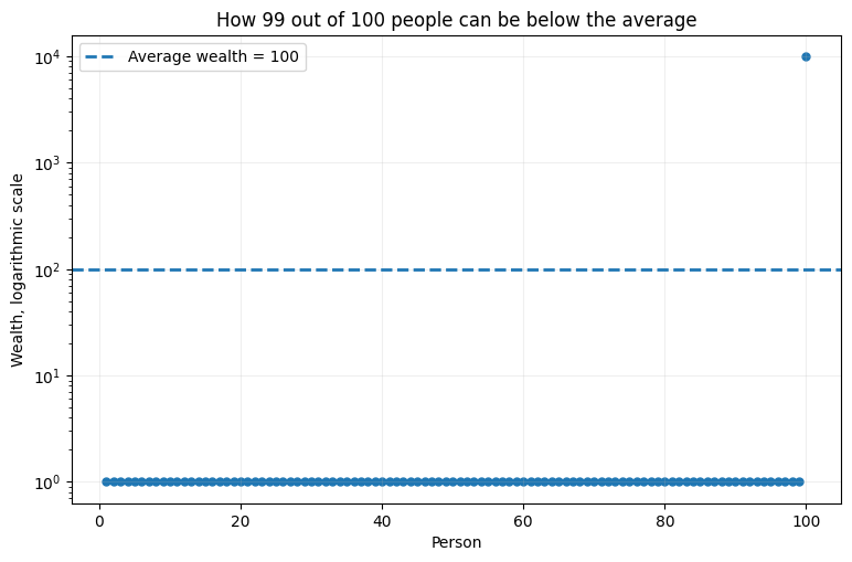
I deliberately made the simplest possible toy economy.
There are 100 people.
Ninety-nine people each own €1.
One person owns €9,901.
Total wealth is €10,000.
Average wealth is therefore €100.
So:
99 people: €1
1 person: €9,901
-------------------
average: €100
Ninety-nine percent of people are below average.
There is nothing mathematically strange about that.
“Average” does not mean “middle.”
It means:
One extreme person can move that number almost arbitrarily far away from what nearly everyone possesses.
This is exactly why the sentence:
can be badly misleading when the distribution is extremely skewed.
The mean isn't lying.
You're asking it a question it wasn't designed to answer.
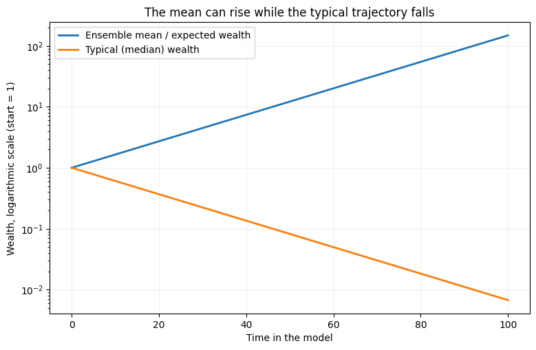
Now look at the second graphic above.
That gets even closer to Peters.
The upper line is expected, ensemble-average wealth.
The lower line is typical wealth.
They start together.
Then one goes up and the other goes down.
How can average wealth increase while the ordinary trajectory gets poorer?
Because rare trajectories become so enormous that they more than compensate for enormous numbers of mediocre trajectories.
Imagine one million people.
999,999 people each end up around €1.
One extraordinary trajectory reaches €1 trillion.
The total wealth is dominated by that one trajectory.
So the average can be around €1 million even though almost nobody has remotely close to €1 million.
That's the trick.
Now make the process continue.
The right tail gets wider.
The rare winners get rarer relative to the whole population, but their values become exponentially more extreme.
So you get the apparently paradoxical result:
In wealth dynamics, the mean becomes more and more prosperous while becoming less and less representative of almost anyone actually living inside the system.
This explains individual economic decay as ensemble statistics look "better".
The first graph is the most important. At the beginning, about half the population is below the expected wealth level. As the multiplicative process runs, that proportion rises.
Why?
Because the distribution is not merely moving. It is stretching.
Imagine everyone begins here:
Time 0
●●●●●●●●●●●●●●●●●●●●
roughly equal
Then everyone receives independent percentage gains and losses.
After some time:
Later
●●●●●●●●●●●●●●● ●● ● ●
poor / ordinary rich very rich
Much later:
Much later
●●●●●●●●●●●●●●●●●●●●●●●●● ● ● ●
almost everyone extreme tail
The huge conceptual point is that wealth is multiplicative.
Suppose two people both get lucky.
One currently has €10.
One currently has €10 million.
A 20% positive shock gives the first person €2.
It gives the second person €2 million.
So once trajectories separate, subsequent percentage changes occur on radically different bases.
The distribution therefore keeps broadening.
And because wealth cannot symmetrically extend below zero in this simple model, the broadening becomes extraordinarily skewed in ordinary euro terms.
In log-wealth space, the distribution looks much more like a symmetric bell.
But when you transform back into actual wealth, the right-hand tail gets stretched enormously.
That is the central geometry:
LOG WEALTH
/\
/ \
/ \
_______/____________\_______
fairly symmetric
becomes something like:
ACTUAL WEALTH
███████████████████▇▆▅▄▃▂▂▁▁▁▁.........................tiny tail
but tail values are ENORMOUS
Most people occupy the dense mass on the left.
Very few people occupy the far-right tail.
But the far-right values become so enormous that they dominate the arithmetic average.
And that brings us to the third graphic.
I deliberately made the simplest possible toy economy.
There are 100 people.
Ninety-nine people each own €1.
One person owns €9,901.
Total wealth is €10,000.
Average wealth is therefore €100.
So:
99 people: €1
1 person: €9,901
-------------------
average: €100
Ninety-nine percent of people are below average.
There is nothing mathematically strange about that.
“Average” does not mean “middle.”
It means:
Add everyone's wealth together and divide by the number of people.
One extreme person can move that number almost arbitrarily far away from what nearly everyone possesses.
This is exactly why the sentence:
“The average person has X”
can be badly misleading when the distribution is extremely skewed.
The mean isn't lying.
You're asking it a question it wasn't designed to answer.
Now look at the second graphic above.
That gets even closer to Peters.
The upper line is expected, ensemble-average wealth.
The lower line is typical wealth.
They start together.
Then one goes up and the other goes down.
How can average wealth increase while the ordinary trajectory gets poorer?
Because rare trajectories become so enormous that they more than compensate for enormous numbers of mediocre trajectories.
Imagine one million people.
999,999 people each end up around €1.
One extraordinary trajectory reaches €1 trillion.
The total wealth is dominated by that one trajectory.
So the average can be around €1 million even though almost nobody has remotely close to €1 million.
That's the trick.
Now make the process continue.
The right tail gets wider.
The rare winners get rarer relative to the whole population, but their values become exponentially more extreme.
So you get the apparently paradoxical result:
The probability of being anywhere near the expectation gets smaller even while the expectation itself keeps growing.


